Relative Hybrid Topology Protocol#
Overview#
The relative free energy calculation approach calculates the difference in
free energy between two similar ligands. Depending on the ChemicalSystem
provided, the protocol either calculates the relative binding free energy
(RBFE), or the relative hydration free energy (RHFE).
Further information on constructing chemical systems to define thermodynamic cycles,
see ChemicalSystems, Components and Thermodynamic Cycles
In a thermodynamic cycle, one ligand is converted into the other ligand by alchemically transforming the atoms that vary between the two ligands. The transformation is carried out in both environments, meaning both in the solvent (ΔGsolv) and in the binding site (ΔGsite) for RBFE calculations and in the solvent (ΔGsolv) and vacuum (ΔGvacuum) for RHFE calculations.

Thermodynamic cycle for the relative binding free energy protocol.#
Scientific Details#
This RelativeHybridTopologyProtocol is based off the Perses implementation.
The Hybrid Topology approach#
The RelativeHybridTopologyProtocol uses a hybrid topology approach to represent the two
ligands, meaning that a single set of coordinates is used to represent the
common core of the two ligands while the atoms that differ between the two
ligands are represented separately. An atom map defines which atoms belong
to the core (mapped atoms) and which atoms are unmapped and represented
separately (see Creating atom mappings). During the alchemical transformation, mapped atoms are switched
from the type in one ligand to the type in the other ligands, while unmapped
atoms are switched on or off, depending on which ligand they belong to.
Note
In this hybrid topology approach, all bonded interactions between the dummy region and the core region are kept. As pointed out by Fleck et al. [1], this can lead to systematic errors if the contribution of the dummy group does not cancel out in the thermodynamic cycle (no separability of the partition function). We are currently working on fixing this issue.
The lambda schedule#
The protocol interpolates molecular interactions between the initial and final state of the perturbation using a discrete set of lambda windows. A function describes how the different lambda components (bonded and nonbonded terms) are interpolated.
Only parameters that differ between state A (lambda=0) and state B (lambda=1) are interpolated.
In the default lambda function in the RelativeHybridTopologyProtocol, first the electrostatic interactions of state A are turned off while simultaneously turning on the steric interactions of state B. Then, the steric interactions of state A are turned off while simultaneously turning on the electrostatic interactions of state B. Bonded interactions are interpolated linearly between lambda=0 and lambda=1. The lambda_settings lambda_functions and lambda_windows define the alchemical pathway.
A soft-core potential is applied to the Lennard-Jones potential to avoid instablilites in intermediate lambda windows.
Both the soft-core potential functions from Beutler et al. [2] and from Gapsys et al. [3] are available and can be specified in the alchemical_settings.softcore_LJ settings
(default: gapsys).
Simulation overview#
The ProtocolDAG of the RelativeHybridTopologyProtocol contains the ProtocolUnits from one leg of the thermodynamic
cycle.
This means that each ProtocolDAG only runs a single leg of a thermodynamic cycle and therefore two Protocol instances need to be run to get the overall relative free energy difference, ΔΔG.
If multiple protocol_repeats are run (default: protocol_repeats=3), the ProtocolDAG contains multiple ProtocolUnits of both vacuum and solvent transformations.
Simulation Steps#
Each ProtocolUnit carries out the following steps:
Parameterize the system using OpenMMForceFields and Open Force Field.
Create an alchemical system (hybrid topology).
Minimize the alchemical system.
Equilibrate and production simulate the alchemical system using the chosen multistate sampling method (under NPT conditions if solvent is present).
Analyze results for the transformation (for a single leg in the thermodynamic cycle).
Note: three different types of multistate sampling (i.e. replica swapping between lambda states) methods can be chosen; HREX, SAMS, and independent (no lambda swaps attempted). By default the HREX approach is selected, this can be altered using simulation_settings.sampler_method (default: repex).
Simulation details#
Here are some details of how the simulation is carried out which are not detailed in the RelativeHybridTopologySettings:
The protocol applies a LangevinMiddleIntegrator which uses Langevin dynamics, with the LFMiddle discretization [4].
A MonteCarloBarostat is used in the NPT ensemble to maintain constant pressure.
Getting the free energy estimate#
The free energy differences are obtained from simulation data using the MBAR estimator (multistate Bennett acceptance ratio estimator) as implemented in the PyMBAR package. In addition to the MBAR estimates of the two legs of the thermodynamic cycle and the overall relative binding free energy difference, the protocol also returns some metrics to help assess convergence of the results, these are detailed in the multistate analysis section.
Analysis#
As standard, some analysis of the each simulation repeat is performed. This analysis is made available through either the dictionary of results in the execution output, or through some ready-made plots for quick inspection. This analysis can be categorised as relating to the energetics of the different lambda states that were sampled, or to the analysis of the change in structural conformation over time in each state.
Energetic and replica exchange analysis#
These analyses consider the swapping and energetic overlap between the different simulated states to help assess the convergence and correctness of the estimate of free energy difference produced.
Description |
Example |
|---|---|
MBAR overlap matrix. This plot is used to assess if the different lambda states simulated overlapped energetically. Each matrix element represents the probability of a sample from a given row state being observable in a given column state. Since the accuracy of the MBAR estimator depends on sufficient overlap between lambda states, this is a very important metric. This plot should show that the diagonal of the matrix has some “width” so that the two end states are connected, with elements adjacent to the diagonal being at least 0.03 [5]. |

|
Replica exchange probability matrix (for replica exchange sampler simulations only). Similar to the MBAR overlap matrix, this shows the probability of a given lambda state being exchanged with another. Again, the diagonal of this matrix should be at least tridiagonal wide for the two end states to be connected. |

|
Forward and reverse convergence of free energy estimates. Using increasingly larger portions of the total data, this analysis calculates the free energy difference, both in forward and backward directions. In this analysis, forward and backward estimates that agree within error using only a fraction of the total data suggest convergence [5]. |

|
Timeseries of replica states. This plot shows the time evolution of the different system configurations as they are exchanged between different lambda states. This plot should show that the states are freely mixing and that there are no cliques forming. |

|
Structural analysis#
If a protein was present, these analyses first center and align the system so that
the protein is considered the frame of reference.
Further analysis can be performed by inspecting the simulation.nc and hybrid_system.pdb files,
which contain a multistate trajectory and topology for the hybrid system respectively.
These files can be loaded into an MDAnalysis Universe object using the openfe_analysis package.
Description |
Example |
|---|---|
Ligand RMSD. This produces a plot called |
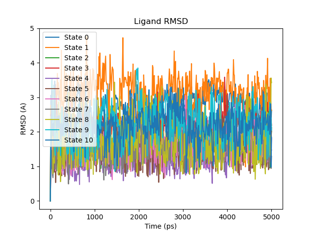
|
Ligand COM drift. For simulations with a protein present, this metric gives the total distance of the ligand COM
from its initial starting (docked) position. If this metric increases over the course of the simulation (beyond 5
angstrom) it indicates that the ligand drifted from the binding pocket, and the simulation is unreliable.
This produces a plot called |

|
Protein 2D RMSD. For simulations with a protein present, this metric gives, for each lambda state, the RMSD of the protein structure over time, using each frame analysed as a reference frame, to produce a 2 dimensional heatmap. This plot should show no significant spikes in RMSD (which will appear as brightly coloured areas). |

|
See Also#
Setting up RFE calculations
Tutorials
Cookbooks
API Documentation